
Gravity surveys · Buyer's guide
Gravity Survey for Mining: Ground, Airborne, Gradiometry
A gravity survey maps density, not ore. Ground crews read stations on a grid; aircraft fly gravity or gradiometer lines. Match spacing to the target, ask for noise figures, and compare quotes on one design.
Key takeaways
- Anomalies that matter in mineral work run from under 1 mGal to several tens of mGal, against a total field near 980,000 mGal (USGS SIR 2010-5070-I).
- Zonge advises ground station spacing no wider than the target and ideally one to two times finer; Australia’s national database spans 11 km to 50 m spacing (Geoscience Australia).
- At a 1 km wavelength, a published comparison gives about 10 mGal RMS for airborne gravimetry and 0.1 mGal RMS for a Falcon gradiometer (Dransfield, 2007).
- Falcon is flown by Xcalibur: a 280 km2 Quebec survey on 100 m lines (Nov 2025) and a 14,727 line-km Michigan job on 500 m lines (Oct 2026).
- No public price list exists, so the calculator takes your own quote figures; compare bids on the same spacing.
In this article
- What a gravity survey measures and what it can find
- Ground gravity survey: stations, spacing and corrections
- Airborne gravity and gradiometry: how they differ
- Providers of airborne gravity gradiometry surveys
- Ground or airborne: which should you buy
- Which targets respond to gravity
- What a gravity survey costs and how to budget
- How to brief a contractor
- Use public gravity data and satellite imagery first
- From anomaly to drill target
- Frequently asked questions
A gravity survey measures tiny changes in the pull of gravity at the surface to find rock that is denser or lighter than its surroundings. Explorers use it to map buried intrusions, faults and basins, and to look for dense ore bodies such as massive sulphide. On the ground, a crew reads a gravimeter at stations on a grid. From the air, an aircraft carries a gravimeter or a gradiometer along closely spaced lines. The USGS describes gravity and magnetic surveys as relatively inexpensive ways to cover large areas of ground (USGS Fact Sheet FS-239-95), but the right method, spacing and contractor depend on what you hold and what you need to find.
This guide is for licence and claim owners, consultants and investors who need to decide whether to buy a gravity survey, which type to buy and how to compare bids. It explains the physics in plain words, shows how station spacing and line spacing drive the size of the job, lists the companies with checkable airborne gravity or gradiometry work, gives a budget calculator with inputs you set yourself, and ends with a contractor checklist and answers to common questions.
What a gravity survey measures and what it can find
Gravity changes from place to place because rocks differ in density. The USGS explains that higher gravity values sit over denser rock and lower values over lighter rock, and that mafic rocks, which hold dense minerals, often show as gravity highs while basin sediments show as lows (USGS). The survey does not see ore directly. It sees a density contrast, and you decide whether the contrast could be caused by something you want.
The signals are very small. Gravity at the surface is about 980,000 milligals (mGal), while the anomalies that matter in mineral work typically run from less than one mGal to several tens of mGal (USGS Scientific Investigations Report 2010-5070-I). One mGal equals 10 micrometres per second squared (Geoscience Australia Record 2004/18). That is why surveys need precise instruments and careful corrections.
A real example shows the scale. The Ovoid nickel-copper-cobalt deposit at Voisey’s Bay in Labrador is associated with a residual gravity anomaly of about 4 mGal, according to the USGS occurrence model for magmatic nickel-copper deposits (USGS SIR 2010-5070-I). The same report notes that picking out a deposit-related anomaly needs careful separation from the signal of other sources, which is the main job of the interpreter.
Bouguer anomaly in one paragraph
Raw readings are not maps. Crews correct them for the Earth tide, instrument drift, latitude, elevation (the height correction), the mass of rock between the station and sea level (the Bouguer correction), Earth curvature and nearby topography (the terrain correction). The USGS lists these steps in its explanation of the gravity method and uses a standard reduction density of 2.67 g/cm3 for the complete Bouguer anomaly (USGS Open-File Report 02-353). The result, the complete Bouguer anomaly, is the map most buyers receive. The reduction density is a choice, so ask the contractor which value was used and test others where relief is steep.
Ground gravity survey: stations, spacing and corrections
A ground gravity survey uses a relative gravimeter, an instrument with a mass on a spring that stretches more where gravity is stronger. The USGS says a relative meter can measure gravity to about 0.01 mGal in roughly five minutes at a station, and each survey is tied back to a known base station in the absolute gravity network (USGS FS-239-95, 1997). Modern meters are faster. Zonge International says it runs LCG-6 gravimeters and uses Scintrex CG-5 meters where higher precision is needed, with geodetic-grade GPS for station position and elevation (Zonge International). Elevation matters because a few centimetres of height error moves the corrected value, so ask for the GPS method and its stated accuracy.
Chart
Gravity stations needed per square kilometre
Square grid, by station spacing
Choosing station spacing
Spacing should match the target. Zonge advises that station spacing generally should not exceed the lateral extent of the target and is ideally one to two times finer than the target’s dimension. A body 400 metres across therefore needs stations at 200 to 400 metres or closer. Regional surveys are far coarser. Geoscience Australia reports that national regional gravity coverage runs from about 11 kilometres between stations over much of northern and western Australia to 1.5 kilometres in Victoria, while some detailed surveys have stations as close as 50 metres (Geoscience Australia, gravity project).
A small historical program shows a practical design. In 1977 Newmont and its partner laid out a reconnaissance grid of three 10 km lines spaced 2.5 km apart on a South Australian licence, read ground magnetics at 250 m intervals and then took 98 gravity stations at 250 m intervals on the same grid (South Australian SARIG record for EL 326). The gravity peak was used to site the first stratigraphic test hole. The lesson still holds: a modest grid tied to a drill decision beats a large grid with no decision attached.
Station count grows with the square of how fine you go. Halving the spacing multiplies the stations by four, and the chart below shows the counts per square kilometre. Field days follow the same curve, which is why contractors quote by station and by day rate.
What a ground survey can do well
Ground gravity works well where you hold a defined block and need a sharper picture than regional data give. Zonge lists structural mapping, lithology changes, alteration mapping and support for direct detection in favourable massive sulphide settings among its uses, and says gravity deliverables include contoured complete Bouguer maps, horizontal gradient and first-derivative maps, and 3D inversion where the scope includes modelling. Its page cites an 800-station survey at the Eastside gold project in Nevada reported by A2Gold in September 2025. Ground work is slower than flying, and the USGS notes that until recently gravity surveying for mineral exploration relied on ground acquisition, which increased time and cost (USGS SIR 2010-5070-I).
Airborne gravity and gradiometry: how they differ
Airborne work comes in two kinds. An airborne gravimeter measures the vertical pull of gravity, as a ground meter does, but from a moving aircraft that is constantly accelerating. An airborne gravity gradiometer measures how that pull changes with distance, using a set of paired accelerometers that cancel most of the aircraft’s motion. Geoscience Australia notes that gradients are given in eotvos units (Eo), where 1 Eo equals 10 to the power of minus 9 per second squared, or 0.1 mGal per kilometre.
Chart
Flight-line spacing in published gradiometry surveys
Metres between flight lines, selected surveys
The full gravity gradient is a tensor with nine components, of which five are independent, according to the BHP Billiton geophysicist Mark Dransfield in a paper for the Exploration 07 conference (Dransfield, 2007). The vertical component is the one most easily tied to geology. Gradient data are sharper at small scales than gravimeter data, so they pick out edges and small bodies, while gravimeters are better at long-wavelength, regional features.
Accuracy: gradiometer against gravimeter
Dransfield compares the two on one scale. Airborne gravimetry typically has an error of 10 mGal RMS at a wavelength of 1 kilometre, falling to 1 mGal RMS at 3.5 kilometres. A Falcon gradiometer flown in a Cessna Grand Caravan has an error of 0.1 mGal RMS at 1 kilometre, a hundredfold improvement, and the advantage shrinks until the two are about equal near 20 kilometres at 0.45 mGal RMS. That is the reason gradiometry is used for prospect-scale targets and gravimetry for regional mapping.
The two main gradiometer designs published noise figures for survey data flown in a Grand Caravan: Falcon at 2.5 Eo RMS filtered to a 300 metre wavelength at 55 metres per second, and Air-FTG at 3.5 Eo RMS filtered to an 800 metre wavelength at 60 metres per second (Dransfield, 2007). These are figures for specific test surveys from around 2007 and are not guarantees for your block. Ask any contractor for the noise it expects at your line spacing, speed and terrain.
Platform, speed and height
Resolution improves when the aircraft flies slower and lower. Dransfield reports that fixed-wing Caravans typically fly at 55 to 65 metres per second (about 120 knots) at 80 to 100 metres above ground in gentle terrain, and that helicopter Falcon surveys can fly lower and slower. At the Ekati diamond property in Canada, a helicopter survey flown at 50 metre line spacing, 50 metres above ground and 30 metres per second resolved a known kimberlite pipe that the earlier fixed-wing survey, flown at 100 metre spacing and 80 metres clearance, did not show. Terrain also matters: the largest signal in a gradient survey is often the topography, and Dransfield shows that elevation errors in the public SRTM satellite terrain data could produce correction errors of up to 21 Eo in one Zambian example, which is why a good survey includes laser or high-quality terrain data. The chart below compares line spacings in published surveys.
Providers of airborne gravity gradiometry surveys
The global supply of airborne gradiometry is small, and it is narrower than for magnetics or electromagnetics. There is no official register, so any list is a sample. The table covers companies for which a dated, checkable statement exists of airborne gravity or gradiometry work. It is not a ranking, and Farmonaut has no commercial link to any company named.
| Company | System | Checkable facts |
|---|---|---|
| Xcalibur Multiphysics | Falcon airborne gravity gradiometer (fixed-wing) | Named by Falco Resources in November 2025 to fly a planned 280 km2 survey on 100 m lines in the Noranda Camp, Quebec, and contracted for a 14,727 line-km survey in Michigan (October 2026) |
| Bell Geospace | Air-FTG full tensor gradiometer | Says on its home page (counter shows 26 years, so figures likely date from about 2020) it has acquired more than 2 million line-km in 530 surveys across 50 countries; its mining page says it owns three Basler BT-67 aircraft with built-in gradiometry, gravity and magnetics |
| Sander Geophysics | AIRGrav airborne gravimeter | Developer of the AIRGrav airborne gravimeter (presented at a 2004 workshop). Flew the first airborne gradiometer survey, a Falcon survey for BHP Billiton in October 1999; the 1999 flight was a contract for BHP Billiton, so ask whether gradiometry is on offer today |
Xcalibur Multiphysics and the Falcon system
Falcon was developed by BHP and Lockheed Martin and flew the first airborne gradiometer survey in October 1999 (Dransfield, 2007). Xcalibur Airborne Geophysics, in operation since 2002, bought the CGG Multiphysics businesses, without the multi-client data library, in a deal GeoExpro reported in June 2021, and named the combined group Xcalibur Multiphysics (GeoExpro, June 2021). Recent client releases show Falcon surveys planned and contracted. They are forward-looking, and Xcalibur’s role here rests on those dated releases and a 2021 trade report, so ask the company for current specifications. Falco Resources said in November 2025 that Xcalibur would fly a fixed-wing Falcon survey on a 100 metre line grid over 280 square kilometres of its Noranda Camp holdings in Quebec to look for shallow volcanogenic massive sulphide targets (Falco news release via INN). On those numbers the flight lines add up to about 2,800 line-kilometres before tie lines, which is simple arithmetic from the release and not a figure the company stated.
In October 2026, Pulsar Helium said it had signed Xcalibur for a gradiometry and magnetic survey of 14,727 line-kilometres at its Falcon project in Michigan, a helium exploration project, with 500 metre line spacing, 5,000 metre tie lines and a planned height of about 165 metres above ground (Crux Investor). The contrast between 100 metre and 500 metre spacing shows how survey design follows the target and the budget.
Bell Geospace and the Air-FTG system
Bell adapted a full tensor gradiometer built for ships to fly in aircraft, and its first commercial airborne survey flew in early 2003 (Dransfield, 2007). Its home page says it has provided full tensor gradiometry to the oil and gas and mining industries since 1994 and lists mineral exploration uses that include locating mineralised contacts and faults, interpreting porphyries, diatremes and channelised placers, and finding volcanogenic massive sulphide deposits (Bell Geospace, mining). Its home page also says it offers feasibility studies to predict how useful a survey would be and what it might cost, which is worth requesting before you commit.
Sander Geophysics
Sander Geophysics flew the first airborne gradiometer survey for BHP Billiton in the Bathurst Camp of New Brunswick in October 1999 (Dransfield, 2007). It is also the developer of AIRGrav, an airborne gravimeter, whose design was presented in a Geoscience Australia workshop volume in 2004 (Geoscience Australia Record 2004/18). A gravimeter fits a broad regional picture; ask whether a gradiometer or gravimeter is being offered for your target.
Ground or airborne: which should you buy
The two are tools for different stages. Airborne work covers large blocks fast and without access problems, and it is the usual way to rank ground across a whole property. Ground work gives point readings you control, suits a small block and can run under trees, in steep valleys or where aircraft cannot fly low. Use the table to match the choice to your question.
Chart
Error of airborne gravity measurements by wavelength
Error in mGal RMS, Falcon flown in a Cessna Grand Caravan; data from about 2004-2007
| Question | Better fit | Why |
|---|---|---|
| Rank a licence of tens to hundreds of square kilometres | Airborne gradiometry | Fast coverage on regular lines; Falco’s survey covers 280 km2 on 100 m lines |
| Sharpen one anomaly before a drill program | Ground gravity | Station spacing can be tuned to the target, as in the Zonge guidance of one to two times finer than target width |
| Map a region with no prior data | Airborne gravimetry or public data | Long-wavelength features; national databases already hold regional data |
| Small, near-surface or narrow target | Low and slow gradiometry, or ground | Lower height and speed raise signal and resolution (Dransfield, 2007) |
| Dense forest, cliffs or no road access | Airborne | No ground crew; ground work is slow where access is hard |
If you already hold magnetic data, gravity adds a second, independent view. A magnetic survey responds to magnetic minerals such as magnetite and pyrrhotite, while gravity responds to total density, so the pair separates dense non-magnetic bodies from magnetic ones. Our guide to geomagnetic survey specifications covers the magnetic side, and the guide to geophysical methods for mining compares gravity with the other methods.
Which targets respond to gravity
Gravity works best where the target is much denser or lighter than its host and is big enough to give a signal at the surface. The record gives several kinds of examples.
- Volcanogenic massive sulphide. Dransfield says these deposits typically have a good gravity response because of their high density, and that ground gravity has been used extensively to find them. The first airborne gradiometer survey covered part of the Bathurst Camp, including the Heath Steele and Stratmat deposits, and gravity highs correspond to zones of mineralisation there.
- Iron-oxide copper-gold. The Candelaria survey in Chile led to the Santo Domingo Sur discovery, which Dransfield calls the most advanced project that is a gradiometer discovery as of 2007. Magnetic data had identified more than 70 target areas, 18 were tested by reverse circulation drilling between February 2003 and May 2005, and three returned encouraging IOCG mineralisation.
- Kimberlites. Diamond exploration has been the largest single target of airborne gradiometry. At Ekati the survey was flown at 100 metre line spacing and 80 metres clearance over 39,000 line-kilometres in three months, and a later helicopter system detected more than 90 percent of the known pipes in the areas it flew.
- Concealed copper-uranium-gold. A South Australian government record says the Olympic Dam deposit was discovered in 1975 by reconnaissance drilling of coincident gravity and magnetic highs, beneath roughly 350 metres of cover (Anderson, 1980, SARIG).
- Nickel sulphide. The Ovoid at Voisey’s Bay carries a residual anomaly of about 4 mGal, but the USGS says a nickel target needs very careful separation from other density sources.
Gold is a special case. Gold grains are too few to change density, so a gravity survey for gold maps the host rocks, intrusions, faults and alteration that control it, and in some settings the sulphides that travel with it. Zonge lists structural and alteration mapping as the main uses in mineral work. The same is true of many other metals: gravity is a map of the setting, not an assay.
What a gravity survey costs and how to budget
No official price list for ground or airborne gravity exists. Quotes depend on the number of stations or line-kilometres, terrain, access, aircraft type, mobilisation distance and the processing you order. Contractors say as much, and Zonge states that daily production depends on spacing, terrain, access and the repeatability required. Do not budget from an old per-station figure. Ask for a written quote based on your own polygon and spacing, and compare quotes only when they use the same design.
The calculator below turns your own numbers into a station count, a rough field cost and the number of field days for a ground grid. Prices are inputs: use today’s price from your contractor quotes. For airborne work the same logic applies in line-kilometres. Take the area in square kilometres, multiply by 1,000 and divide by the line spacing in metres. A 100 square kilometre block at 100 metre spacing needs about 1,000 line-kilometres, and at 500 metre spacing about 200, before tie lines and turns.
Calculator
How many gravity stations and what budget for my block?
Enter your own block size, spacing and the rates from your quotes.
- Station cost before processing: $37,500
- Total with mobilisation: $47,500
- Field days: 6.2
Example values only, not a benchmark or a price list. Prices are inputs: example, use today’s price from your contractor quotes. Stations = area in m2 divided by spacing squared on a square grid; it ignores base ties, repeats, terrain surveying, processing and interpretation.
How to brief a contractor
A short written brief makes bids comparable and prevents disputes over what was delivered. Include these points.
- The question. State the target: its size, depth and expected density contrast against the host rock.
- The block. Send a KML or shapefile of the survey boundary and any no-fly or no-access areas.
- The design. Station spacing or line spacing, tie-line spacing, flying height and speed for airborne work, and the base-station plan for ground work.
- Precision. The noise or repeatability you expect at that spacing, stated as a number with its filter wavelength.
- Positioning. The GPS method and the accuracy of station elevation.
- Processing. The corrections applied, the reduction density, the terrain model and how terrain errors are checked.
- Deliverables. Located data in a standard format, complete Bouguer or gradient grids, a processing report and, if wanted, 3D inversion. Zonge lists contoured Bouguer maps, derivative maps and inversion outputs among its deliverables.
- Safety and access. Landowner or claim-holder permission, aviation approvals and permits are yours to arrange or confirm in writing.
For related guidance on hiring crews, see our guide to airborne geophysical survey platforms and contractors.
Use public gravity data and satellite imagery first
Before paying for a survey, check what already exists. Geoscience Australia’s national database holds more than 1.5 million point gravity observations from more than 2,300 surveys, and the open-file data can be downloaded online by region (Geoscience Australia). The USGS releases station data for its survey areas, such as the survey behind one 30 by 30 minute California quadrangle map with more than 2,300 data points (USGS Open-File Report 02-353). Many state and provincial surveys hold similar data. Public data are usually coarse, so they help with regional setting and not with a 100 metre target.
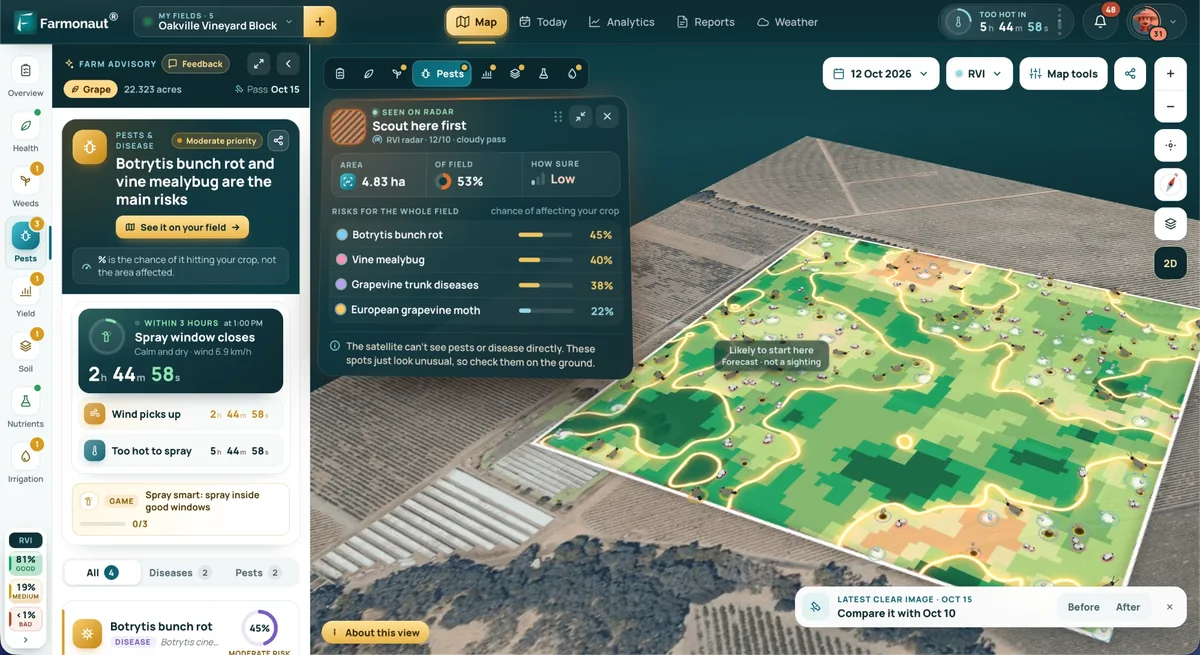
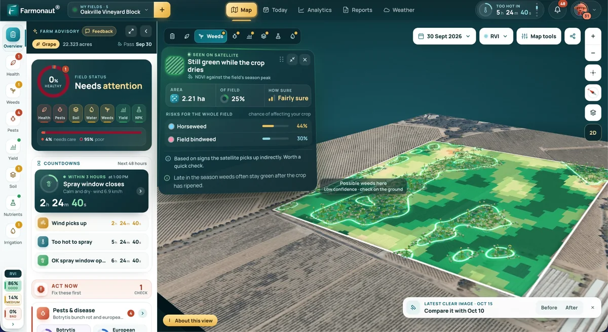
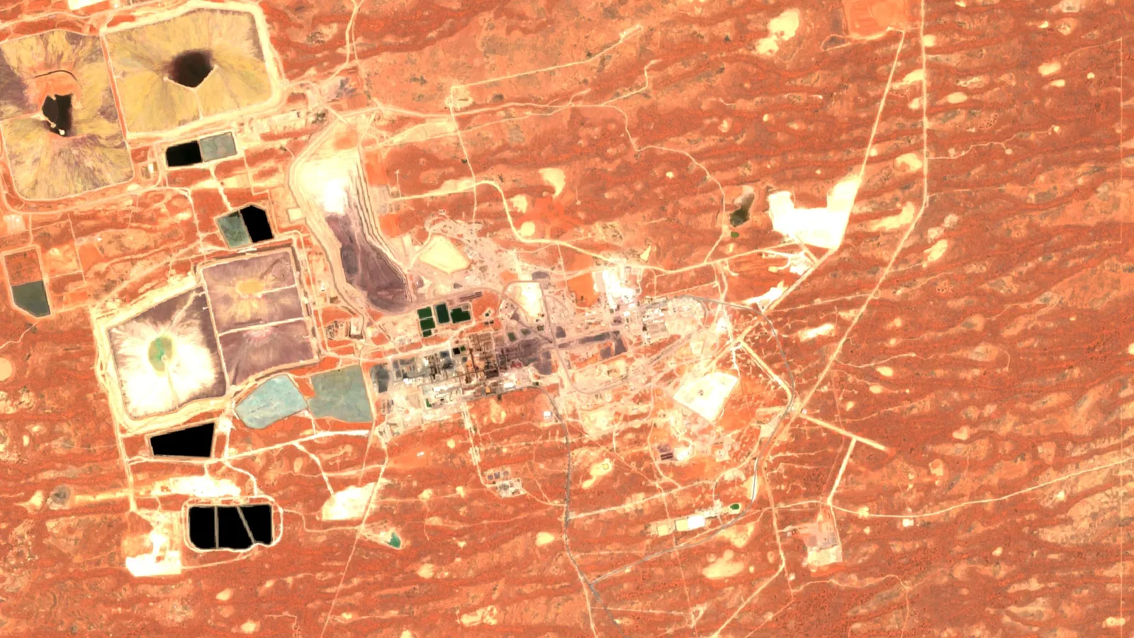
Satellite imagery is a different screen. It maps surface alteration, iron-stained rock and structure, so it can show where a gravity program is most likely to earn its cost. It cannot measure density. The Farmonaut mining service maps these surface signals from satellite data on a licence polygon, and it can help you place a first gravity grid, but it does not replace one. For a short plain-language explainer of the instrument families used in remote sensing, watch the video below.
▶ Plain explainer of remote sensing for mining and the instrument families used to measure ground from a distance. · 2:01
From anomaly to drill target
A gravity map is the start of interpretation, not the end. The USGS notes that anomaly maps carry information about rock density and also about the depth and distribution of the sources, so one anomaly can have several explanations. A common workflow is to remove the regional trend to get a residual, calculate derivatives that sharpen edges, model the body with a density contrast you can defend, and test the model against magnetics, geology and any drilling. Zonge lists inversion and residual analysis as optional deliverables.
Then rank the targets. Gravity highs that sit on structure, with a matching magnetic or geochemical signature and an accessible depth, move up. Anomalies explained by known dense rock, such as a mafic dyke on the surface map, move down. Rank by the cost and chance of a drill test before you sign for any hole. Our guide to picking an exploration drilling contractor covers the next step, and the video below shows how targets are ranked into a drill order.
Present the result honestly. A gravity anomaly is an exploration target, not a resource, and it does not meet the reporting rules for mineral resources under JORC or NI 43-101 until drilling and an estimate by a competent or qualified person have been done.
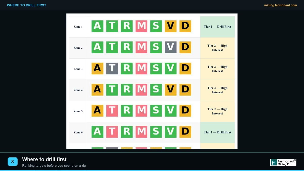
▶ Shows how thirteen satellite targets are ranked into a drill order that a programme can defend. · 2:19
Frequently asked questions
What is a gravity survey in mineral exploration?
It is a survey that measures small changes in the pull of gravity to map differences in rock density below the ground. A gravity high suggests denser rock, such as mafic intrusions, and a low suggests lighter rock, such as basin sediments (USGS FS-239-95).
How much does a gravity survey cost?
There is no public price list. Cost depends on station or line-kilometre count, terrain, access, aircraft and processing. Use the calculator on this page with your own quote figures, and compare bids that use the same spacing.
What is a ground gravity survey?
A crew reads a gravimeter at stations on a grid, with GPS for position and elevation, and ties the readings to a base station. The data are corrected to a complete Bouguer anomaly map. Spacing is usually set at one to two times finer than the width of the target, per Zonge.
What station spacing should I use?
Match it to the target. Zonge advises spacing no wider than the target’s lateral extent and ideally one to two times finer. Detailed surveys in Australia’s national database go as close as 50 metres, while regional coverage runs from 11 kilometres to 1.5 kilometres between stations.
What is gravity gradiometry?
Gradiometry measures how the pull of gravity changes over short distances, in eotvos units. It gives sharper detail on edges and small bodies than gravimetry, and it is the main airborne method for prospect-scale density mapping (Dransfield, 2007).
What is the difference between airborne gravity and gradiometry?
An airborne gravimeter measures gravity itself and is best for long wavelengths. A gradiometer measures its gradient and has lower noise at short wavelengths. At a 1 kilometre wavelength, one published comparison (Dransfield, 2007, using 2004-era data) gives about 10 mGal RMS for airborne gravimetry and 0.1 mGal RMS for Falcon. Ask contractors for current figures.
Who provides airborne gravity gradiometry surveys?
The companies with checkable recent or historical work are Xcalibur Multiphysics (Falcon), Bell Geospace (Air-FTG) and Sander Geophysics (the AIRGrav gravimeter; it also flew the first Falcon gradiometer survey in 1999). Request written specifications from each, because systems, aircraft and availability change.
Can gravity find gold?
Not directly. Gold is too sparse to change rock density. Gravity maps the host rock, intrusions, faults and alteration associated with gold, and sometimes the sulphides that accompany it, so use it with geology, magnetics and geochemistry.
How deep can a gravity survey see?
There is no single depth. Signal falls as depth rises and grows with the size and density contrast of the body. Olympic Dam was found beneath about 350 metres of cover (Anderson, 1980), but a small body needs to be much shallower. Ask a modeller to test your target before you buy.
Do I need permission to run a gravity survey on my claim?
Yes, in most places. Check what your licence or claim allows, get landowner or surface-rights consent where it is needed, and arrange aviation approvals for airborne work. Rules differ by country and state, so confirm them with the regulator.
This page is for information only. It is not investment or legal advice, and companies are named for orientation, not as recommendations. Confirm access, permission and aviation rules with the regulator, and confirm services and prices with each contractor.
Farmonaut mining
Screen your ground from space before you book a survey
Request a quote to map alteration and structure on your licence from satellite data and decide where a gravity grid should go.
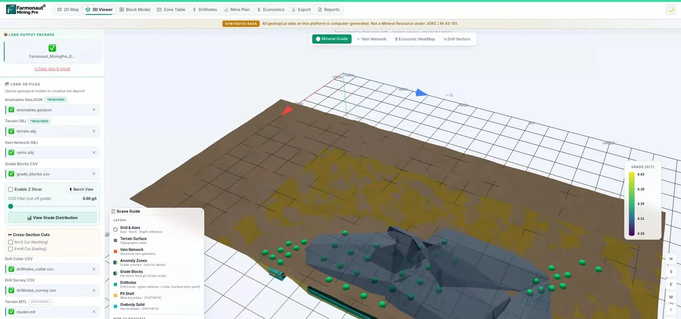
Mining Pro sample view, synthetic data
Sources
- USGS, Introduction to Potential Fields: Gravity, Fact Sheet FS-239-95 (1997): pubs.usgs.gov
- USGS, Explanation of the gravity method, Open-File Report 02-353: pubs.usgs.gov
- USGS, Occurrence model for magmatic nickel-copper deposits, SIR 2010-5070-I: pubs.usgs.gov
- Dransfield, Airborne Gravity Gradiometry in the Search for Mineral Deposits, Exploration 07 (2007): 911metallurgist.com
- Geoscience Australia, Record 2004/18, Airborne Gravity 2004 abstracts: ga.gov.au
- Geoscience Australia, Australian National Gravity Database: ga.gov.au
- Zonge International, ground gravity method: zonge.com
- Bell Geospace, Air-FTG for mineral exploration: info.bellgeo.com
- GeoExpro, Xcalibur expansion (18 June 2021): geoexpro.com
- Falco Resources, Noranda Camp airborne gravity gradiometry survey (5 Nov 2025), via INN: investingnews.com
- Crux Investor, Pulsar Helium contracts Xcalibur (5 Oct 2026): cruxinvestor.com
- Geological Survey of South Australia, Anderson (1980), Magnetic and gravity interpretation on the Stuart Shelf: catalog.sarig.sa.gov.au
- Geological Survey of South Australia, EL 326 Danae Hill exploration record: catalog.sarig.sa.gov.au
Discussion
Questions, corrections or field experience? Share them below. First-time comments are reviewed before they appear, and your email is never published.
No comments yet. Be the first to add a question or your experience.

 African Venture Partners Holding
 Congo Mining Solutions
 Mining SARL
 SenGold Invest SAS
 Sania Corporation
 Sean Mining Limited
 NTS Group (Pty) Ltd
 Mine4Africa
 Lithspo Minerals Limited
 Tintina Mining Group
 Dalgety Minerals Pty Ltd
 Vortex Minerals Pty Ltd
 Faith At Work (Pty) Ltd
 Geotech Mining Solutions plc
 Vulcan International Limited
 Kidepo Associates
 GKY Mining
 Alkimy SARL
 Double A Trading
 GemSprout Metals Limited