
Exploration targeting · Method guide
Mineral Prospectivity Mapping: Data, GIS Workflow, Models
A prospectivity map scores every cell of an area by how closely it matches known deposits of one type. Geoscience Australia’s national copper-gold model puts 91.7% of known deposits in 8.3% of the continent. Here are the data, GIS steps, models and tests.
Key takeaways
- Prospectivity maps combine geology, geochemistry, geophysics and satellite layers to rank ground for one deposit type (Scientific Reports, 2026).
- Geoscience Australia’s national iron oxide copper-gold model captures 91.7% of known deposits and occurrences in 8.3% of the area (Geoscience Australia, 2024).
- Sentinel-2 has 10 m visible and 20 m shortwave infrared bands; ASTER shortwave data from April 2008 onward is unusable (Google Earth Engine catalog; NASA Earthdata).
- A higher AUC is not always the better map: one study’s grid-search model scored 0.90 against 0.95 for Bayesian tuning but had the best-calibrated probabilities (Scientific Reports, 2026).
- A map is a ranking tool, not a resource estimate; test it on held-out deposits before drilling decisions.
In this article
- What a prospectivity map shows and what it does not
- Seven steps from raw data to a ranked target map
- Choosing the deposit model and study area
- Data layers: what to collect and where to find it
- Remote sensing layers for alteration and structure
- Geochemical anomaly mapping in GIS
- Building evidence layers that models can use
- Knowledge-driven, data-driven and machine learning models
- What machine learning studies show for prospectivity mapping
- How to test a prospectivity map before you trust it
- From scores to targets: reading the map
- Common mistakes that ruin a prospectivity map
- When a satellite screen is enough, and when you need a full model
- Frequently asked questions
A mineral prospectivity map is a ranked picture of where a chosen deposit type is most likely to occur, built by combining geological, geochemical and geophysical layers in a GIS (geographic information system) and scoring every cell of the map. The method is also called mineral potential mapping or prospectivity modelling. Its purpose is narrowing the search: Geoscience Australia’s national iron oxide copper-gold model, for example, places 91.7% of known deposits and occurrences inside 8.3% of the continent (Geoscience Australia, 2024). This guide covers the data you need, a seven-step GIS workflow, the main model families, how to test a map and the mistakes that make a pretty map useless, for licence owners, consultants and investors who must decide where the next dollar of exploration goes.
A prospectivity map is a ranking tool, not a resource estimate. It does not say how much metal is in the ground, and it never replaces sampling or drilling. It tells you which parts of a licence or district look most like known deposits, so that cheaper work (mapping, soil sampling, a geophysical line) goes there first.
What a prospectivity map shows and what it does not
Every prospectivity map answers one narrow question: how closely does each cell look like the ground around known deposits of one type? A cell is a square of the map, often 100 m to 1 km across for district work. Each cell carries a score between 0 and 1 (or a class from low to high) built from evidence layers such as distance to a fault, rock type, a geochemical anomaly or an alteration index from satellite images.
Chart
Share of known deposits against share of area
National iron oxide copper-gold model, Australia
The method works because ore deposits form where several conditions overlap. A Scientific Reports study describes the aim plainly: integrate geological, geochemical and geophysical datasets to outline areas with a high probability of hosting deposits, and so reduce exploration cost and uncertainty (Scientific Reports, 2026). Geoscience Australia’s national assessments follow the same logic. They build mappable spatial proxies for each component of a mineral system, meaning the full set of processes that make a deposit, and then combine them with a knowledge-driven approach so that areas where the favourable criteria coincide stand out (Ford and others, Geoscience Australia).
Three limits are worth stating early. A map can only rank what its inputs describe, so a district with no geophysics will be scored on geology alone. A map is built for one deposit model: an orogenic gold map says nothing about porphyry copper. And a high score is a reason to look, not a discovery. Readers who want the geology behind each deposit model can start with our guide to types of ore deposits.
Seven steps from raw data to a ranked target map
Most published prospectivity studies follow the same order, whether the final model is a simple overlay or a neural network. The steps below are the sequence a consultant would follow on a licence or a district of several thousand square kilometres.
Infographic
From raw data to ranked targets in seven steps
- 1Pick the deposit modelName the deposit type and its host rock, structure and alteration.
- 2Set area and cell sizeInclude barren ground; match the coarsest layer.
- 3Collect and clean dataGeology, geochemistry, geophysics, satellite, elevation.
- 4Build evidence layersDistance, density, index or class, rescaled to one scale.
- 5Weight and combineExpert weights, statistics or machine learning.
- 6Test the mapHold-out deposits, capture rate, calibration.
- 7Rank targetsAdd tenure, access and cover, then plan field work.
- Pick the deposit model. Write down what you are looking for (for example, carbonate-hosted lead-zinc or epithermal gold) and the features that deposits of that type share: host rock, structure, alteration, geochemical signature.
- Set the study area and cell size. The area should be large enough to contain barren ground as well as known deposits. The cell size should match the coarsest data you will use, not the finest.
- Collect and clean the data. Geology, structure, geochemistry, geophysics, satellite images and a digital elevation model, all in one coordinate system.
- Build evidence layers. Turn each dataset into a map of one idea, such as distance to a fault or an iron-oxide ratio, and rescale it so layers can be compared.
- Weight and combine the layers. Use expert weights, statistics from known deposits or a machine-learning model.
- Test the result. Check how well the map picks out deposits it was not trained on, and whether the high-scoring areas make geological sense.
- Turn scores into targets. Cut the map into ranked areas, add access, tenure and cover, and decide on field work.
The same seven steps are drawn in the infographic below. The sections that follow take them in turn, with the most space on data, evidence layers and testing, because that is where most projects succeed or fail.
Choosing the deposit model and study area
The deposit model decides everything downstream, so be specific. “Gold” is too broad: an epithermal gold system, an orogenic gold belt and a placer gold fan have different hosts, structures and surface signatures. Our guide to ore deposit types sets out the main families, and the Argentine gold study in the literature shows why it matters: the authors first reviewed the geology of porphyry, epithermal and orogenic gold districts and then built separate targeting models for epithermal and orogenic systems (Ford and others, Ore Geology Reviews, 2015).
Define the study area around the geology, not the licence boundary. A model trained only inside one licence has few deposits and no contrast. A district-wide area, with a few dozen known occurrences and plenty of barren ground, gives the statistics something to learn from. You can then clip the final map back to your own tenure.
Fix the cell size now. A cell much finer than your coarsest layer invents precision that is not there. Regional work usually settles on the resolution of the geochemistry or geophysics, not the satellite pixel.
Data layers: what to collect and where to find it
Five families of data feed most models. The table lists each family with typical sources and the main thing to watch. Public geoscience data is often enough for a first-pass map, and in the United States the Earth Mapping Resources Initiative is one example of a programme built to supply it. The USGS describes it as a partnership with state geological surveys to improve knowledge of the geologic framework through geologic mapping and airborne geophysical and lidar surveys, with the aim of identifying areas that may hold undiscovered critical minerals (USGS Fact Sheet 2019-3007).
Chart
Pixel size of common open layers
Metres per pixel; smaller is finer
| Layer family | Typical sources | What it adds | Watch for |
|---|---|---|---|
| Geology and structure | National and state geological survey maps, 1:100,000 to 1:250,000 | Host rocks, faults, contacts | Map scale; faults drawn from sparse outcrop |
| Geochemistry | Stream sediment, soil and rock chip databases from surveys and company reports | Pathfinder and target elements | Different labs, methods and sampling dates |
| Geophysics | Airborne magnetic, radiometric and electromagnetic surveys | Buried structure, intrusions, alteration | Line spacing; survey vintage and levelling |
| Remote sensing | Sentinel-2, Landsat, ASTER, radar | Alteration, iron oxides, lineaments, terrain | Cloud, vegetation, soil and weathering cover |
| Known deposits | Survey mineral occurrence databases, company data | Training points and test points | Locations in the wrong place; missing small occurrences |
Geophysics deserves a note. Magnetic and radiometric surveys see through thin cover that hides the surface geology, and they usually come with the best structural information in a district. Our guide to geomagnetic survey specifications explains line spacing and flying height, which decide how fine a feature the data can resolve. Geological map scale matters in the same way, and our page on geological mapping methods and scales covers how to read what a map can and cannot show.
Spatial detail varies a lot between open satellite products. Sentinel-2 records visible and near-infrared light at 10 m and its two shortwave infrared bands at 20 m (Google Earth Engine catalog, Sentinel-2). Landsat 9 surface reflectance is 30 m in every band (Google Earth Engine catalog, Landsat 9), and the Copernicus GLO-30 elevation model is also 30 m (Google Earth Engine catalog, Copernicus DEM). The chart shows how these compare. A model built on a 1 km grid can use any of them, but a 100 m grid may start to show the difference.
Remote sensing layers for alteration and structure
Satellite images support prospectivity maps in two ways. They map the surface expression of alteration, where hot fluids changed the rock around a deposit, and they map structure, through lineaments and terrain. Shortwave infrared bands matter most for alteration, because clay minerals, micas and carbonates absorb light there. If the idea is new to you, the short video below explains spectral signatures and why shortwave infrared does the work.
There is one trap with a well-known sensor. The ASTER instrument carried six shortwave bands that earlier prospectivity work relied on, but NASA reports that its shortwave infrared detectors are no longer functioning because of high detector temperatures, with data from April 2008 onward unusable and the visible and thermal data unaffected (NASA Earthdata, ASTER SWIR anomaly). For recent shortwave infrared coverage, Sentinel-2 and Landsat each offer two bands, with ASTER archive scenes from before the failure still useful for a fixed point in time.
Simple band ratios remain the workhorse. A Scientific Reports lead-zinc study used ASTER ratios of bands 14/12 to highlight silica alteration and bands 2/1 to highlight iron oxides, then turned each into a distance-to-alteration map (Scientific Reports, 2026). Treat any ratio as a hypothesis. A study of volcanogenic massive sulphide gossans in the Asmara Belt of Eritrea found that a ratio method plus supervised classification could separate oxidised gossans from the widespread hematitic laterites that look similar in multispectral images (PLOS One, 2026). The lesson is general: iron staining is not ore, and every ratio needs a field check on both mineralised and barren ground.
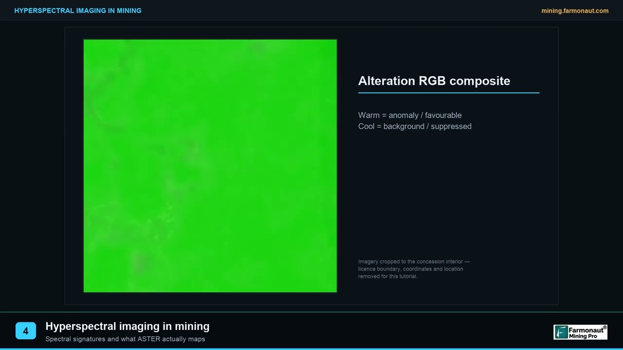
▶ Explains spectral signatures, why shortwave infrared does the work, and what it cannot tell you. · 1:49
Geochemical anomaly mapping in GIS
Geochemical data is the most direct layer, and also the most error-prone. The standard reference, Emmanuel Carranza’s Geochemical Anomaly and Mineral Prospectivity Mapping in GIS (Elsevier, 2009), is organised in three parts: how GIS data models connect to mapping, GIS-based methods for setting reliable anomaly thresholds, and spatial analysis and data integration for modelling where minerals are likely to occur (James Cook University record of the book). The same order works as a checklist for your own project.
First, clean the data. Put every sample in one coordinate system, check units (ppm against percent), handle values below detection limit in one stated way, and separate sample types (stream sediment, soil, rock chip) because they do not behave alike. Our guide to geochemical survey design covers how samples are taken, which decides how far you can trust them.
Second, set a threshold. A background value and an anomaly threshold separate normal ground from unusual ground. A simple start is the mean plus two standard deviations of the log-transformed values, but one threshold for a whole district is rarely right, because background changes with rock type. More careful methods, such as fractal and catchment-based analysis of stream sediment anomalies, are among the methods the book covers.
Third, map it properly. Stream sediment samples represent the whole catchment upstream, not the point where they were taken, so a point map of stream data misleads. Soil data can be interpolated into a surface, but only where sample spacing is tight enough to justify it. Finally, convert the anomaly into an evidence layer: a distance-to-anomaly map or a score that rises with the number of pathfinder elements above threshold.
Building evidence layers that models can use
An evidence layer is one dataset recoded into a map of one geological idea. Most are made in a few ways: distance to a feature (a fault, a contact, a favourable rock unit), density of a feature (faults per square kilometre), an index (an alteration ratio), or a class (rock unit A, B or C).
All layers then need a common scale. The lead-zinc study above converted proximity to favourable limestone, fault density and proximity to alteration into a 0 to 1 fuzzy scale using a logistic function, so that a value of 1 always meant “most favourable” (Scientific Reports, 2026). Rescaling is not a cosmetic step. A model that sees one layer in metres and another in parts per million will misweigh them unless they are brought to a common footing.
Two checks save trouble. First, test for redundancy: two layers that carry the same information (for example, distance to a fault and fault density) will double count that evidence in a simple overlay. Second, avoid layers that only exist near known deposits, such as detailed soil grids that were sampled because a deposit was already known. Those layers describe where people looked, not where ore is.
If you use QGIS, most of these steps (distance rasters, density, reclassification, raster calculator) are built in. Our page on QGIS for geologists compares exploration workflows in QGIS and ArcGIS.
Knowledge-driven, data-driven and machine learning models
The model combines the layers into one score. The choice depends mostly on how many known deposits you have.
| Approach | How weights are set | Needs known deposits? | Best when |
|---|---|---|---|
| Boolean or index overlay | Geologist assigns scores and weights | No | Frontier ground with no deposits |
| Fuzzy logic | Expert membership values, combined with fuzzy operators | No | A good deposit model, few data |
| Weights of evidence, frequency ratio | Statistics from deposits inside and outside each layer class | Yes, a dozen or more | A district with a modest deposit count |
| Logistic regression | Fitted from deposit and barren cells | Yes | Many layers, moderate deposit count |
| Random forest, SVM, neural networks | Learned from labelled cells | Yes, plus barren examples | Larger datasets with many layers |
| Hybrid | Expert criteria, then statistics to prune and weight | Some | National or regional maps |
Knowledge-driven and data-driven methods are often combined. The Argentine gold study generated both weights-of-evidence and fuzzy logic maps from public digital data, and found that both highlighted known deposits inside mineralised districts and also flagged highly prospective areas with no known deposits (Ford and others, 2015). Geoscience Australia’s national iron oxide copper-gold model is a hybrid: the team tested which criteria from earlier regional models were statistically important, removed five and added four new or revised criteria from recent geoscience datasets (Geoscience Australia, 2024).
The simplest statistic from known deposits is the frequency ratio. For one layer class (say, “within 500 m of a fault”), divide the share of known deposits that fall inside the class by the share of the study area the class covers. A value of 1 means the class is no better than chance; 5 means deposits are five times more common than random. The calculator below computes it, and also shows how much of the area you can set aside and what share of deposits you would keep.
Calculator
How good is one evidence layer? Frequency ratio calculator
Enter your own cell and deposit counts for one layer class (for example, within 500 m of a fault).
- Share of area in the class (%): 8.3
- Share of deposits captured (%): 91.7
- Area you can set aside (%): 91.7
Example values only, not a benchmark: the defaults are rounded to mirror the 91.7% of deposits in 8.3% of the area reported by Geoscience Australia (2024). The frequency ratio is the share of deposits inside the class divided by the share of area it covers; 1 means no better than chance. No prices are used.
What machine learning studies show for prospectivity mapping
Machine learning is popular, and it needs honest handling. The central problem is labels: confirmed deposits are rare, so a training set may hold a few dozen positive points against many thousands of cells. The Scientific Reports study states the issue bluntly: most algorithms rely on large quantities of labelled data that are rarely available in early-stage exploration (Scientific Reports, 2026). Three recent studies show what researchers do about it.
Chart
Four models, almost the same AUC
Porphyry-skarn copper, southern Peru; AUC multiplied by 100, spatial cross-validation
- Pick the model by more than accuracy. The same paper tested two ensemble models with three tuning strategies on one lead-zinc district. One model reached an AUC of 0.95 with Bayesian tuning and 0.90 with grid search, yet the grid-search version gave the most stable, best-calibrated probabilities. The authors conclude that calibration matters more than small accuracy gains when training data is thin.
- Test on separate ground. SRK compared four models for porphyry-skarn copper in southern Peru using spatial cross-validation based on geographic clustering. AUC scores were 0.89 for random forest, 0.912 for a multilayer perceptron, 0.901 for a convolutional network and 0.907 for a graph convolutional network. The perceptron scored highest, but the graph model gave results that were more spatially and geologically coherent (SRK Peru).
- Use the spatial structure. Oxford researchers re-cast exploration data as a graph so that neighbouring areas inform each other. On copper, iron and tin in the southern United Kingdom, graph models improved on tabular models, and the authors recommend training with more barren than mineralised examples (Sihombing and others, Ore Geology Reviews, 2024).
Two further ideas address the label problem directly. Positive-unlabelled learning trains on known deposits only, without pretending the rest are barren: an EarthByte model for porphyry copper in the American Cordillera did this, matched or beat traditional classifiers in North America, but scored poorly in South America, a reminder that a model does not carry over between tectonic settings (EarthByte). Self-supervised pretraining on unlabelled geospatial data, tested on lead-zinc deposits in North America and Australia, is another route (arXiv, GFM4MPM). Neither is a shortcut for a licence owner today, but both explain why a vendor’s claim of “AI targeting” should come with a validation table, not just a colourful map. The video below explains in plain terms what AI does in exploration and how to check a claim.

▶ Explains how AI is used in mineral exploration, where it fails and how to check a claim. · 4:37
How to test a prospectivity map before you trust it
A map that scores well on the deposits it was built from proves little. Four tests give a fair picture.
Chart
AUC changes with the tuning method
Two ensemble models, one lead-zinc district; AUC (1.0 is perfect)
- Capture rate against area. What share of known deposits falls in the top-ranked area, and how big is that area? Geoscience Australia’s 91.7% in 8.3% is this kind of result. A map that captures 50% of deposits in 40% of the area is only a little better than chance.
- Hold-out deposits. Keep some known deposits out of training, then see whether the map finds them. With clustered deposits, split by area, not at random, which is what the SRK study’s spatial cross-validation does.
- Calibration. If the model says 0.8, do about 80% of such cells hold deposits in the test data? The Scientific Reports study treated calibration as a main measure for this reason.
- Geological sense. Look at what drives the score. A high-scoring cluster caused by one noisy layer, such as a cloud edge in an image, is an artefact.
The AUC figure in these studies is the area under the receiver operating characteristic curve. It runs from 0.5 (chance) to 1.0 (perfect ranking). It is useful, but as the two studies above show, a higher AUC does not always mean the better map.
From scores to targets: reading the map
Cut the score surface into a few classes, not a smooth rainbow, and rank the high-score areas by size and by the number of independent layers supporting each one. Then add the practical filters that no model sees: tenure, access, land use, cover thickness and the cost of the first field visit.
Read each target against its drivers. A target supported by structure, alteration and a geochemical anomaly is stronger than one that is high only because it is close to a mapped fault. Also look at the areas the map ranks high but where no deposit is known: these are the new ideas, and also the places where an error would be most costly. The Argentine gold study treated them as exactly that, flagging prospective ground with no known deposits as areas worth testing (Ford and others, 2015). The short video below shows how to read a satellite-based prospectivity surface in an exploration report.
The usual next steps run from cheapest to dearest: desk review, reconnaissance mapping and sampling, a geophysical line, trenching, then drilling. Our overview of mineral exploration stages, methods and timelines lays out that sequence.
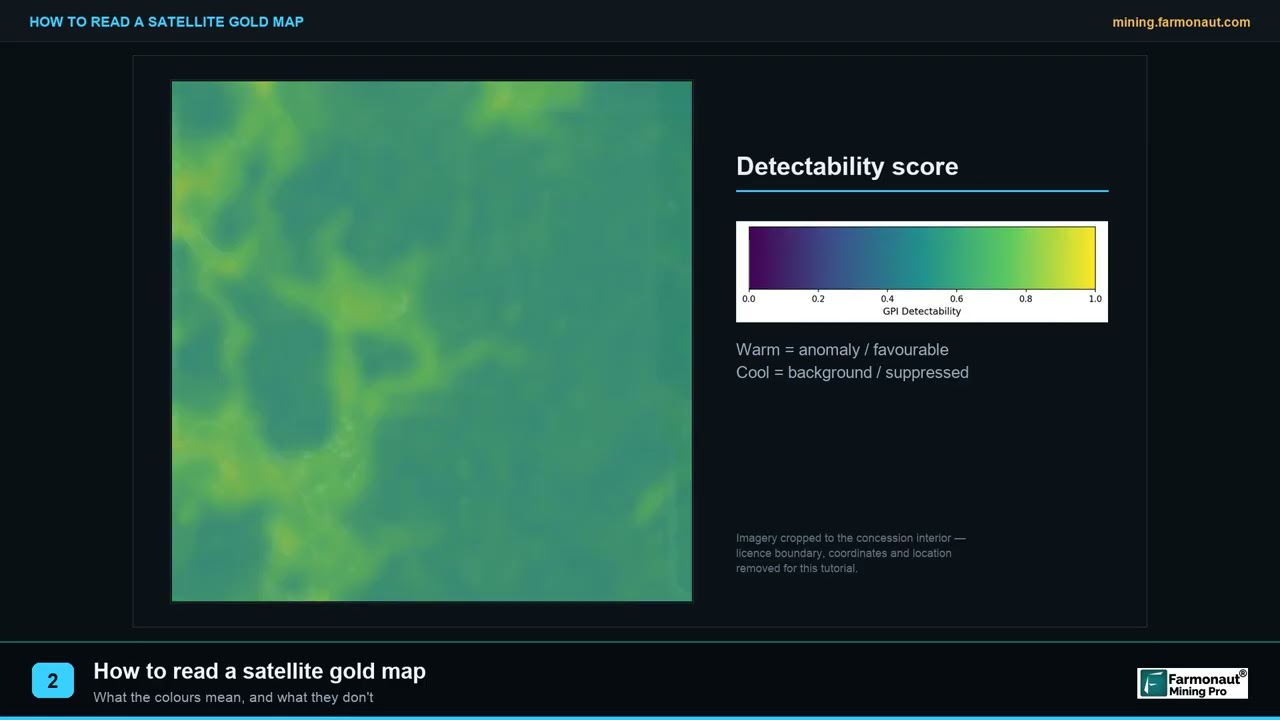
▶ Explains how to read a satellite prospectivity surface in an exploration report. · 1:40
Common mistakes that ruin a prospectivity map
- Circular evidence. Using a layer that was made from the deposits you are trying to predict, such as a geochemical grid sampled only around known mines.
- Too few deposits for the method. Training a neural network on a handful of occurrences. Use an expert-weighted method or a hybrid instead.
- Random test splits on clustered deposits. Nearby deposits end up in both training and test sets and the score looks better than it is.
- One deposit model, many commodities. Mixing deposit types into one set of labels blurs the signal.
- Ignoring cover. Where soil, laterite or sediment hides the bedrock, surface layers describe the cover, not the rock below. The Eritrean laterite example shows how easily weathered ground can imitate an ore signal.
- Stale or mismatched data. Old shortwave infrared archives, surveys flown at wide line spacing, or geological maps at a scale too coarse for the cell size.
- Reporting only the colour map. A map with no capture rate, no test method and no list of layers cannot be checked.
When a satellite screen is enough, and when you need a full model
A full prospectivity model needs a district of known deposits, several data layers and weeks of expert work. For a single licence with sparse data, a satellite screen is often the sensible first step: it maps alteration, structure and terrain from public imagery, and ranks areas for field follow-up. Farmonaut offers satellite mineral screening for areas supplied as KML, KMZ or polygon files, with results in business days rather than months. These are exploration targets, not a resource estimate, and they do not carry any reporting-code status.
A practical order for a licence owner is to start with public geology and geophysics, build or buy a first-pass map, and use field checks to decide whether the licence warrants a full multi-layer model. Satellite screening can also help an investor or buyer judge claims before paying for them. Whatever route you take, ask to see the layers used, the test method and the capture rate.
Frequently asked questions
What is mineral prospectivity mapping?
It is a GIS method that combines geological, geochemical, geophysical and satellite layers to score every part of an area by how likely it is to host a chosen deposit type. The output is a ranked map used to choose where to explore first.
Is mineral potential mapping the same thing?
Yes, in practice. Mineral potential mapping, prospectivity modelling and favourability mapping all describe the same workflow. Some authors use “potential” for the geological probability and “prospectivity” when economic or access factors are also included.
What data do I need for a prospectivity map?
At minimum: a geological map with faults, known mineral occurrences, and one more layer from geochemistry, geophysics or satellite imagery. More independent layers give a better map, provided each one reflects a real feature of the deposit model.
How do I map a geochemical anomaly in GIS?
Clean and level the data, split it by sample type, set a background and a threshold (preferably by rock unit), map stream data by catchment and soil data by interpolation, then convert the anomaly into a distance or score layer for the model.
Which software is best for prospectivity mapping?
Any GIS that handles rasters works: QGIS (open source) or ArcGIS for layer preparation, and Python or R for statistical and machine-learning models. The method matters more than the package.
Which model should I use: weights of evidence, fuzzy logic or machine learning?
Use fuzzy logic or expert scoring when you have few or no known deposits. Use weights of evidence or logistic regression when you have a dozen or more deposits. Use machine learning when you have many labelled examples and spatial cross-validation. Hybrid models are common for large regions.
How accurate are prospectivity maps?
It depends on data and testing. Published studies report AUC values from about 0.89 to 0.95, and Geoscience Australia’s national copper-gold model places 91.7% of known deposits in 8.3% of the area. These are test results on known deposits, not a promise that new deposits sit in the high-scoring cells.
Can satellite images alone make a prospectivity map?
They can rank ground by alteration and structure, which is useful for a first screen. Without geology, geochemistry and geophysics, a satellite-only map cannot separate ore-related alteration from similar-looking weathering, as the Eritrean laterite example shows.
How many known deposits do I need to train a model?
There is no fixed number. Studies show that machine-learning models become unstable with very few labels, so a small count favours expert-weighted or fuzzy methods, or approaches such as positive-unlabelled learning built for sparse labels.
Does a prospectivity map replace drilling?
No. It ranks ground for cheaper work first. Only sampling and drilling can confirm grade and tonnage, and any resource estimate must follow the reporting code that applies to your project.
This page is general information for licence owners and consultants, not investment or technical advice. Confirm tenure, access rights and any permit requirements before you do field work.
This page is for information only. It is not investment or technical advice. A prospectivity map ranks ground for follow-up; it is not a resource estimate. Confirm tenure, access and permit rules before field work.
Farmonaut mining
Screen your licence area from space
Request a quote to have your licence screened with satellite data so you know which ground to check first.
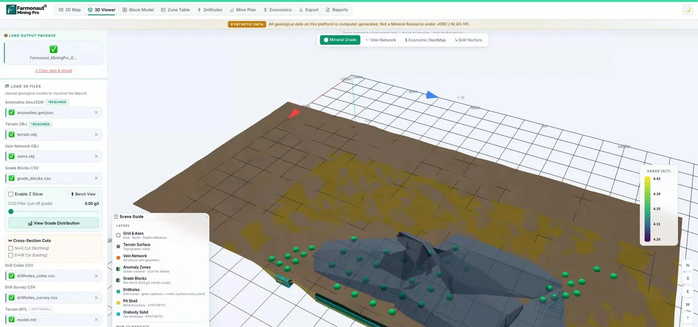
Mining Pro sample view, synthetic data
Sources
- Geoscience Australia, First national mineral system assessment of Australia’s iron oxide copper-gold potential (2024): ecat.ga.gov.au
- Ford and others, Sediment-hosted mineral potential mapping of Australia (Geoscience Australia): zenodo.org
- Scientific Reports, Ensemble machine learning strategies for mineral prospectivity mapping under data scarcity (2026): nature.com
- Ford and others, Porphyry, epithermal and orogenic gold prospectivity of Argentina (2015): researchonline.jcu.edu.au
- Carranza, Geochemical Anomaly and Mineral Prospectivity Mapping in GIS (Elsevier, 2009), JCU record: researchonline.jcu.edu.au
- USGS Fact Sheet 2019-3007, The Earth Mapping Resources Initiative: pubs.usgs.gov
- NASA Earthdata, ASTER SWIR anomaly: earthdata.nasa.gov
- Google Earth Engine catalog, Sentinel-2 SR Harmonized: developers.google.com
- Google Earth Engine catalog, Landsat 9 Collection 2 Level 2: developers.google.com
- Google Earth Engine catalog, Copernicus DEM GLO-30: developers.google.com
- PLOS One, Sentinel-2 VMS mineralization mapping in the Asmara Belt, Eritrea (2026): journals.plos.org
- SRK Peru, Porphyry-skarn copper prospectivity mapping with machine learning models: srk.com
- Sihombing and others, Improved mineral prospectivity mapping using graph neural networks (Ore Geology Reviews, 2024): ora.ox.ac.uk
- EarthByte, Spatio-temporal copper prospectivity in the American Cordillera: earthbyte.org
- arXiv, GFM4MPM: Geospatial foundation models for mineral prospectivity mapping: arxiv.org
Discussion
Questions, corrections or field experience? Share them below. First-time comments are reviewed before they appear, and your email is never published.
No comments yet. Be the first to add a question or your experience.

 Huckleberry Garnet LLC
 Dalgety Minerals Pty Ltd
 Vortex Minerals Pty Ltd
 Faith At Work (Pty) Ltd
 Geotech Mining Solutions plc
 Vulcan International Limited
 Kidepo Associates
 GKY Mining
 Alkimy SARL
 Double A Trading
 GemSprout Metals Limited
 Qader Group
 Ileys General Trading
 SG Gold Mining LLC
 VRV Global Pte Ltd
 Omsri International FZE
 G.I.T.T.
 Jaunita Erss Ltd
 Almosi SARL
 SRK Consulting
 Berks Gold Limited
 Mwerezi Minerals Company Limited

 Exploration consultancy · South Africa · Gold